What is this algorithm for?
Documentation references
Inputs and outputs
Spatial partitioning optimization
The triangle set
Data structures
Algorithm
Known limitations
Code repository

[This was originally posted in the Unity forums]

What is this algorithm for?

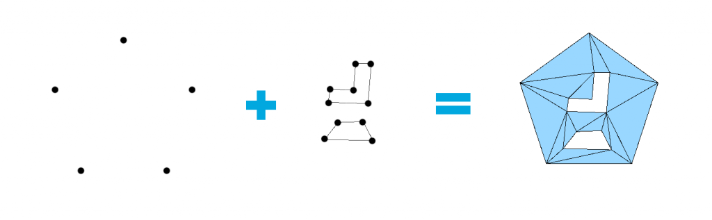
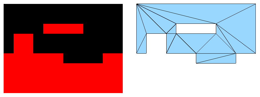
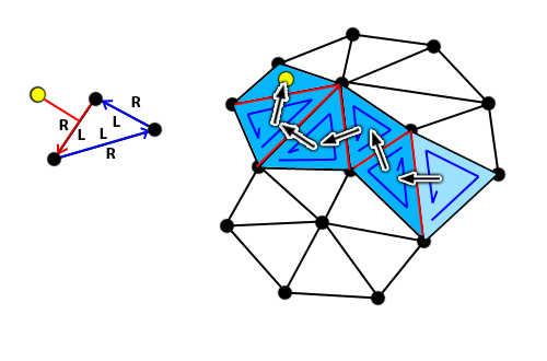
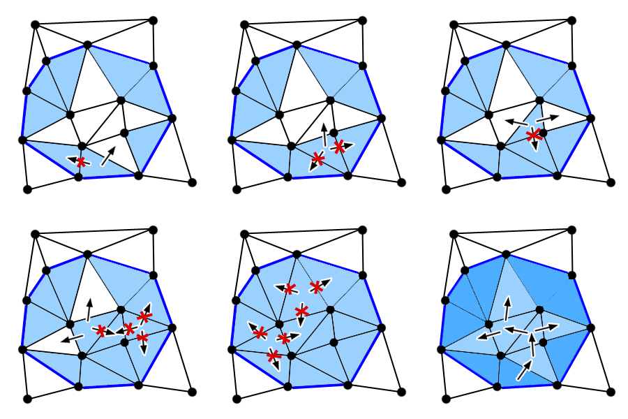
The main purpose of this algorithm is to generate a triangle mesh in which the shape of most of the triangles are as little like a knife (thin and tall) as possible; or, in other words, they tend to be equilateral. The mesh is created from a point cloud and may have holes (other point clouds). Applications are many: terrain geometry, navigation meshes (triangle edges form the edges of a graph used for path-finding), physic colliders (recently, Unity added an option to optimize them)… Below, you can see how I applied the algorithm in the implementation of my 2D navigation mesh, in Unity:

Documentation references

These are the 2 only papers I have used as a base for my implementation:

• A fast algorithm for constructing Delaunay triangulations in the plane (Advanced Engineering Software, Vol. 9 No. 1, 1987), by S. W. Sloan.
• A fast algorithm for generating constrained Delaunay triangulations (Computers and Structures Vol. 47 No. 3, 1993), by S. W. Sloan.

Inputs and outputs

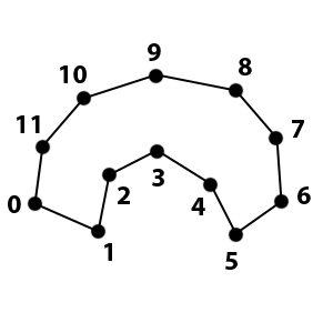
The algorithm expects 2 inputs, the main point cloud to triangulate and, optionally, the shape of the holes, non-connected areas of the triangulated surface that must not contain triangles. All the points must belong to the XY plane. The holes are determined by sorted point sets that form closed polygon outlines (constrained edges), with a minimum of 3 edges. It is not necessary that polygons are convex. 

The result of the algorithm is a list of triangles that belong to the XY plane and fulfill the Delaunay rule. All the points provided in the main point cloud will be present in the resultant triangles unless a hole prevents them from being there. Points provided as the outline of a hole may be included in the result.

Spatial partitioning optimization

Sloan proposes in his papers the construction of a rectangular grid that divides the space occupied by the point cloud in cells in an early stage of the process, with the aim of optimizing a later step, concretely the search-triangle-by-adjacency step. Every cell contains a numerated “bin” in which we deposit points. What this process achieves is to sort all the points by proximity, all the points that belong to the same region of the space are stored together, and the next cell contains a set of points that are as far as the width of a cell.

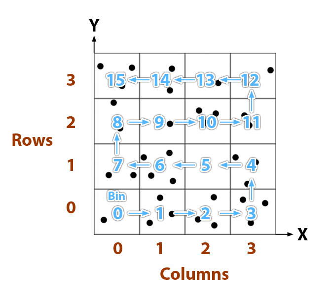
This is how it works:

1. Calculate the boundaries of the point cloud.
2. Determine the amount of columns and rows of the grid. Sloans proposes a MxM grid where M is the fourth root (∜N) of the amount of points in the main point cloud.
3. Reserve a memory buffer to store the M² cells.
4. Every time a point P is added to the grid, calculate the row and column that corresponds to its position relative to the bottom-left corner (0, 0).
   Row = 0.99 x M x Py / GridHeight
   Column = 0.99 x M x Px / GridWidth
5. According to the row and column of the cell that contains the point, calculate the bin number B.
   B = Row x M + Column + 1, when Row is even
   B = (Row + 1) x M – Column, when Row is odd
6. Add the point to the bin (a point list).

As you will read later, when searching for the triangle that contains a point, we use the last created triangle as the first triangle to check; in case that triangle does not contain the new point, we jump to its adjacent; since we will be adding the points to the triangulation in the same order they are stored in the grid, we know that the next point will be near to the last created triangle.
The class PointBinGrid implements this mechanism. It stores an array of point lists (bins).

The triangle set

The algorithm requires to keep track of the vertices in the triangulation, the triangles formed by those vertices and the spatial relation between the triangles, i. e. what triangles are adjacent. All that data is managed by the same entity, the DelaunayTriangleSet class. It also provides some functions to obtain useful processed data, like searching for the triangles that share an edge or calculating which triangles intersect a line. Despite its name, this class knows nothing about the Delaunay condition or triangulation algorithms.

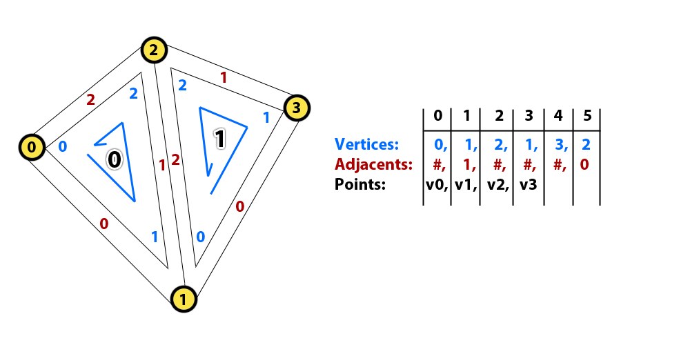
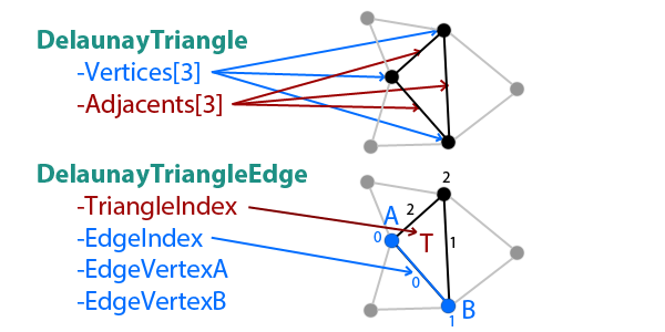
There are 3 arrays in this entity: adjacent triangles (indices), triangle vertices (indices) and points (2D vectors). There is no “array of triangles”, triangles are defined by groups of 3 consecutive indices; for example, the first triangle is defined by the vertices in positions 0, 1 and 2 of the array, whereas the second triangle is defined by the vertices in the positions 3, 4 and 5. So, when we want to access the data of the triangle with number T (starting at zero), we read the array elements T x 3 + 0, T x 3 + 1 and T x 3 + 2.

• Adjacent triangles: It stores the 3 adjacent triangles of a triangle, by their triangle index, in counter-clockwise (CCW) order. The adjacent triangle at the position 0 shares the edge which starts at the vertex 0 and ends at the vertex 1.
• Triangle vertices: It stores the indices of the points in the Points array that form every triangle, in CCW order.
• Points: The actual position of the points in the space, in the order they were added. A point may belong to many triangles. Points are never removed from the triangulation.

A very common operation in this implementation is wrapping around when iterating through the 3 vertices of a triangle. Imagine we are processing the second vertex V₁ (1) of a triangle (0, 1, 2), and you want to modify the other two vertices of the triangle; in order to make the code as generic as possible and avoid IF blocks, you can just add 1 and 2 to the known index, and apply the modulo 3 operation afterwards; in this case, V₂ = (V₁ + 1) % 3 = 2, V₀ = (V₁ + 2) % 3 = 0.

Data structures

In order to make the code more readable and easy to work with, 2 data structures have been defined: DelaunayTriangle and DelaunayTriangleEdge. Both are aimed to be temporary (not persistent) data vehicles when moving packed triangle data among functions. The first contains all the data related to a triangle, which are its vertices (indices) and which are its adjacent triangles; the second represents a single edge of a triangle.

Algorithm

1. Normalization

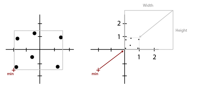
This step is not required but, as Sloan points out, it reduces the lack of precision when rounding off and allows to skip some checks, as we can assume all points will be always between the coordinates [0, 0] and [1, 1].

First, we calculate the bounds of the main point cloud by iterating through all of them and getting the minimum and maximum values for X and Y. Then pick the maximum distance between the height and the width of the bounding box D_max.

Height = Y_max – Y_min
Width = X_max – X_min
D_max = Max(Height, Width)

Finally, for each input point, move it in such a way that it keeps its relative distance to (X_min , Y_min) but as if such bottom-left corner was displaced to [0, 0]; then scale down the point by the maximum size of the bounding box D_max.

X_n = (X – X_min) / D_max
Y_n = (Y – Y_min) / D_max

2. Addition of points to the space partitioning grid

The normalized points are sorted by relative distance using the space partitioning grid. We can add them in any order. Once the points of the grid are added to the Triangle set (in the following steps) this grid will become useless.

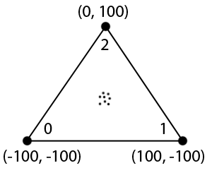
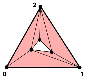
3. Supertriangle initialization

The first triangle in the Triangle set will be a “supertriangle”. We can choose any 3 points as long as the triangle contains all the points. It is preferable to use a very big triangle, even if a smaller one could fit, since that will assure that constrained edges added in the final steps will lay inside of the triangle. Using a supertriangle is convenient as an initialization step for the triangulation process, it avoids the need of performing some initial checks and makes sure the first point we add belongs to a known triangle. I recommend sticking to the triangle proposed in the papers ([-100, -100], [100, -100], [0, 100]). Remember that its vertices must be sorted CCW. This will create 3 points, 3 triangle vertices (0, 1 and 2) and 3 adjacent triangles (#, # and #) in the Triangle set. I will use the symbol ‘#’ to represent “no adjacent triangle” or “undefined” in this document, although in code I use constants with the value -1.

4. Adding points to the Triangle set and Triangulation

The triangulation algorithm operates with one input point at a time and modifies part of the already stored triangle data. It returns the index of the point in the Points array.

4.1. Check point existence

When attempting to add a new point, we first check whether that point already exists; if it does, we just return the index of the position where the point is.

4.2. Search containing triangle

If it is really new, we search for a triangle in the Triangle set that contains it. The first triangle we will check is the last created triangle. For the first point ever added to the set, the first triangle to check will be, obviously, the supertriangle.

For each edge in the triangle, we calculate on which side of the line the point is (in the XY plane). Being the edge formed by vertices A and B, you can use the cross-product between AB and AP. Since vertices are sorted CCW, if the point is on the right side of any of the edges then we are sure that it is not contained in the triangle.

The next triangle to check is the one that shares the same edge we just checked. Once we find a triangle in which the point is on the left side (edge included) of the 3 edges, we stop searching.

4.3. Store the point

Just add it to the Points array of the Triangle set and get its index.

4.4. Create 2 triangles

We join the 3 vertices of the containing triangle to the new point, forming 3 new sub-triangles. We have information about where all the vertices are and which triangles are adjacent to which others. We can do some assumptions too, for example, if we use the new point as the first vertex of every triangle then we can be sure about which is the opposite edge (index 1) and hence which is its adjacent triangle outside of the containing triangle. For the new triangles T, and T₂, contained in T₀:

T₁.vertices = (P, T₀v[0], T₀v[1])
T₁.adjacents = (T₂ , T₀a[0], T₀ )

T₂.vertices = (P, T₀v[2], T₀v[0])
T₂.adjacents = (T₀ , T₀a[2], T₁ )

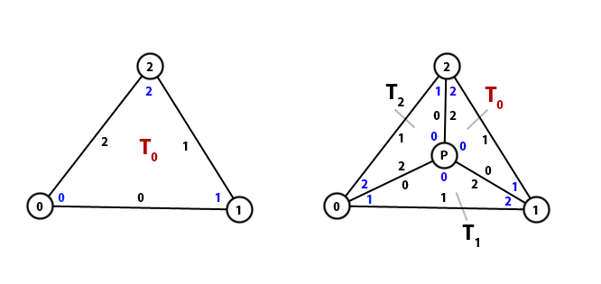
4.5. Transform containing triangle into the third

The containing triangle T₀ is not removed but transformed into the third sub-triangle. Only 3 indices require modification:

T₀.vertices = (P, T₀v[1], T₀v[2])
T₀.adjacents = (T₁ , T₀a[1], T₂ )

Note: I’m using the triangle letters, like T, alternatively as triangle indices, triangle data and groups of 3 points, I hope it does not lead to confusion.

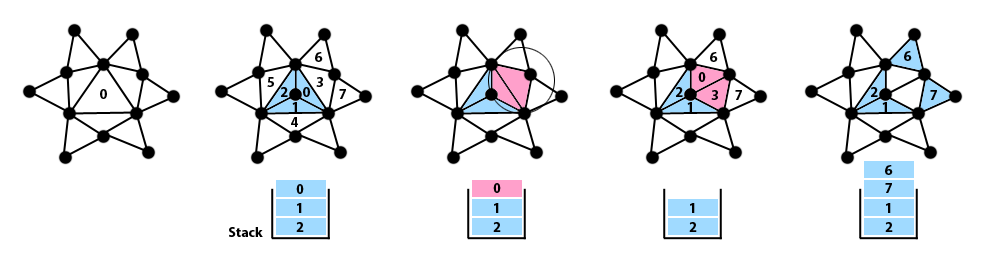
4.6. Add new triangles to a stack

In the next step we are going to use either 2 parallel stacks or 1 stack that contains 2 indices per item: 1) the index of the adjacent triangles that are pending to be checked and 2) the local index (0 to 2) of the edge of those triangles that was shared with a previously processed triangle at the moment they were added to the stack.
The 3 new triangles are added to the stack for a later process step, if they have an adjacent triangle that is opposite to the point P (i. e. if T_na[1] != #). It is assumed that the index of the edge shared with the adjacent triangle, in the three cases, equals 1.

Note: There is a discrepancy here among the 2 documents written by Sloan. One says the 3 triangles must be added whereas the other says only their adjacent triangles (which oppose to P) must.

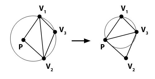
4.7. Check Delaunay constraint

From Sloan’s papers: “The Delaunay constraint stipulates that the diagonal V₁-V₂ is replaced by the diagonal P-V₃ if P lies inside the circumcircle for the triangle V₁-V₂-V₃”. This is something we have to check every time a new triangle is created.

In the previous step we filled the stack with the new triangles. Triangles are processed one at a time. Let’s call the current triangle T_i . We know that the new point is at T_iv[0] because we forced it to be. That is going to be our point P.

We obtain the adjacent triangle T_A that opposes P by reading the value of T_ia[X], where X equals the index of the edge that is stored along with the index of the triangle in the stack.

Then V₁, V₂ and V₃ in the previous wording are T_Av[0], T_Av[1] and T_Av[2], respectively. If P is in the circumcircle of T_A , the diagonal of the quadrilateral formed by both triangles, T_i and T_A, has to be swapped; otherwise, we go back to the beginning of this step and take the next triangle from the stack. Please note that, even after the swap occurs, and no matters how far the swap propagates, the point P will always be T_i [0].

Before swapping the edge, we need to know which of the edges of the adjacent triangle T_A coincides with it. We know the index of the current triangle so it is as simple as iterating through the adjacent triangle indices of T_A until they match. That gives us the edge number E_A (whose value may go from 0 to 2). We use the edge number to know the position of the other 2 adjacent triangles of T_A and we add their indices to the triangle stack, propagating the Delaunay constraint check to the next adjacent triangles until no edge needs to be swapped. The edge shared among T_A and each adjacent triangle is calculated and stored too, in the same order.

Adjacent triangle 1 = T_Aa[(E_A + 1) % 3]
Adjacent triangle 2 = T_Aa[(E_A + 2) % 3]

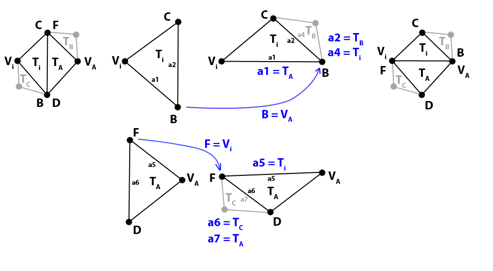
4.8. Swap edges

Basically, if we have a convex quadrilateral formed by 2 triangles T₀(A, B , C) and T₁(C, B, D), this process will generate 2 alternative triangles T₀(A, D, C) and T₁(A, B, D). We just have to perform certain changes in the vertex and adjacency data of both triangles and their adjacents, without reserving nor releasing memory. Technically we are only moving one vertex in each triangle. Before showing the operations, let’s define the local index (0 to 2) of the vertex of T_A that does not belong to the shared edge E_A:

V_A = T_A[(E_A + 2) % 3]

And the same for the index of the opposite vertex in T_i , which we will call V_i . These are the changes to make in all the implied triangles, in order:

T_iv[(V_i + 1) % 3)] = T_Av[V_A ]
T_Av[E_A ] = T_iv[V_i ]
T_Aa[E_A ] = T_ia[V_i]
T,a[V_i ] = T_A
T_ia[(V_i + 1) % 3] = T_Aa[V_A ]
T_Aa[V_A ] = T_i

For the 2 adjacent triangles whose neighbor has changed, we need to know the index of the adjacent triangle that matched their original neighbors, either T_i or T_A, and replace it with the other. The index of the triangles to update are:

T_B = T_ia[(V_i + 1) % 3] → Find T_Ba[n] that matches T_A and replace with T_i
T_C = T_Aa[E_A] → Find T_Ca[m] that matches T_i and replace with T_A

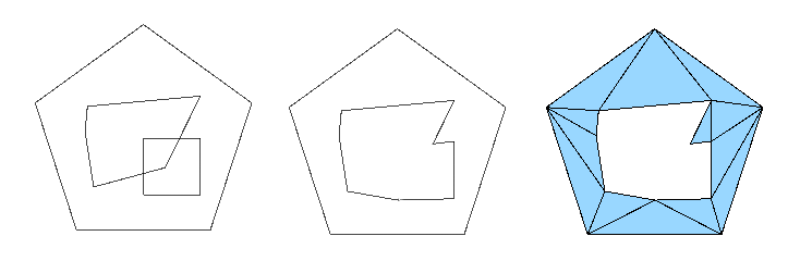
5. Holes creation

A hole is a closed polygon (it is not required that it is convex) described by an array of points H that represent the edges of the outline, sorted CCW. So H[0] → H[1] defines an edge, H[1] → H[2] defines the next edge, and so on. Obviously the last edge is defined by H[H_count – 1] → H[0]. These edges, also known as constrained edges, will be added to the existing triangulation creating new triangles that must satisfy the Delaunay constraint but avoiding to swap the edges that belong to the polygon outline. If there are 2 consecutive coincident points (zero-length edge) in the outline, one of them must be discarded. For each hole, the points of its outline are normalized and added to the triangulation.

5.1. Normalize

The points of the polygon have to be normalized in the same way the main point cloud was, using the same bounds we calculated for those points, so the polygon is moved and scaled accordingly.

5.2. Add the points to the Triangle set

All the points of the outline are added to the Triangle set, one by one, in exactly the same way we did with the main point cloud. The index of every added point has to be stored in an array so we know which point is connected to which other. There is one array per hole. As we add the points, new triangles are generated which may or may not have the edges of the polygon.

5.3. Create the constrained edges

For each hole, we iterate through its vertex indices, defining the constrained edges with pairs of vertices. First, check if the edge already exists, i. e. whether there is a triangle that has the current edge. If so, ignore the edge; otherwise we can proceed to create it.

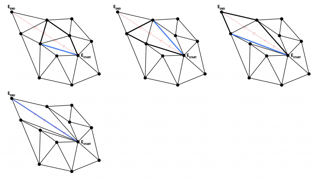
5.3.1. Search for the triangle that contains the beginning of the new edge

In a later step we will calculate which triangle edges intersect the constrained edge but, in order to do that in an optimum way, we need to know which triangle to check the first and follow the trajectory of the line; otherwise we would have to calculate the intersection for every edge in the Triangle set.

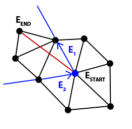
The edge starts at an existing vertex E_START so we search for the index of the vertex in the triangle vertices array of the Triangle set and store the indices of the triangles that have that vertex. Then, for each triangle (V₀, V₁, V₂), we identify at which position the vertex V_i is (0, 1 or 2) and, using that value, we obtain the contiguous edges:

V_i1 = (V_i + 1) % 3
V_i2 = (V_i + 2) % 3
E₁ = V_i → V_i1
E₂ = V_i2 → V_i

Finally we check if the other endpoint of the edge, E_END , is on the left side of both edges E₁ and E₂, and we stop searching if that’s the case. We have found which of all the triangles that share the same vertex contains the first endpoint, E_{START ,} of the future constrained edge.

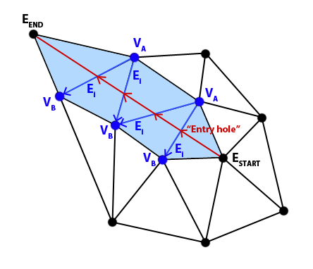
5.3.2. Get all the triangle edges intersected by the constrained edge

For each triangle T_N in the Triangle set, and starting with the triangle that contains E_START , we first check that T_N is not the triangle that contains the other endpoint E_END. Take into account that, normally, the line will intersect 2 edges of every triangle and that, for every triangle, only the “exit hole” is calculated; the “entry hole”, or first intersection, is calculated by the previous checked adjacent triangle, and so on. So the last intersected triangle is a special case, we do not need to check for intersections, it is obvious that the “entry hole” is somewhere and the “exit hole” is its vertex. As you may foresee, as soon as this special case occurs, the process to find intersecting edges finishes and the output list is returned.

For each of the 3 edges in T_N we check if E_END is on the right side, which means the line may intersect that edge. If we find that case, we take note of the index of the current edge E_i (0, 1 or 2) and store the value in another place, let’s call it E_T; this is the tentative edge of the next adjacent triangle. Now we calculate the intersection among the triangle edge and the constrained edge.

If they intersect:

• Store the index of the vertices that form the edge (V_A and V_B) in the output list.
• Use a flag to know when any of the edges of T_N has been crossed. Set it to True.
• Set the next triangle to check

T_N = T_N a[E_i  ]

If they do not intersect, continue iterating through the edges of T_N.

If none of the 3 edges of T_N intersect with the constrained edge (check the flag), then

T_N = T_N a[E_T ].

This process is similar to the search for a triangle that contains a point, we jump from one triangle to its adjacent in the direction of E_END, instead of testing all triangles by brute force.

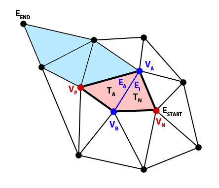
5.3.3. Form quadrilaterals and swap intersected edges

Once we know all the existing edges that obstruct the constrained edge, we iterate through that list with the purpose of removing them until the constrained edge can join E_START and E_END, keeping everything triangulated.

We copy the last element (the 2 indices of the vertices that form the intersected edge, V_A and V_B) and remove it from the list. We use them to search by brute force for a triangle T_N in the Triangle set that has that edge, in that order, and also what is the local index E_i (0, 1 or 2) of the edge in such triangle. We cannot store the triangle index of previous steps to save the cost of this search because triangles may change as we swap edges; but vertices stay the same.

We get the opposite adjacent triangle T_A that shares the same intersected edge, V_A → V_B .

T_A = T_N a[E_i ]

Then we calculate the local index (0, 1 or 2) of the same edge in T_A, by iterating linearly and comparing with V_B (remember that the same edge is flipped in the adjacent triangle), and we also get the vertex V_P of T_A that opposes that edge. If the mentioned comparison is true for the index J, then we can calculate:

E_A = J
V_P = T_Av[(J + 2) % 3]

We now have almost all the information we need for swapping the edge, in case it is necessary. The condition for that is that the quadrilateral formed by the vertices T_Nv[0], T_Nv[1], T_Nv[2] and V_P is convex. If so, we only need one more data, the vertex V_N that opposes the edge in T_N:

V_N = T_N [(E_i + 2) % 3]

We swap the edge V_A → V_B in the same way we did in previous steps. In case the quadrilateral was not convex, the pair V_A-V_B is added back to the first position of the list and the current iteration ends.

The last part of this step is to check whether the swapped edge still intersects the constrained edge. We can obtain the endpoints of the edge, V_C→ V_D easily using a trick. A known consequence of the swap operation is that the local position of the shared edge of the first triangle, in this case T_N, is moved 2 positions forward:

E_i’ = (E_i + 2) % 3

Therefore, the new endpoints are:

V_C = T_Nv[E_i’ ]
V_D = T_Nv[(E_i’ + 1) % 3]

Be careful with not using a cached version of the information related to T_N, it has changed after the swap operation. Now we calculate the intersection between E_START → E_END and V_C → V_D. In order to avoid false positives, if the edges share any vertex then we consider them not intersecting. In case they do intersect, the pair of indices of the vertices V_C and V_D is inserted at the first position of the list of intersected edges; otherwise, we add that information to a list of new edges. The current iteration ends.

5.3.4. Check Delaunay constraint and swap edges

When the algorithm reaches this step, the constrained edge has been already added to the triangulation and there is no other edge obstructing it. For all the new triangles we created, it is necessary to check whether they still fulfill the Delaunay constraint. We iterate through every new edge of the list.

We do not want the constrained edge to be touched anymore so the first thing to do is to discard that the current edge V₁ → V₂ coincides with it.
As we did in a previous step, we search for a triangle T_C that uses V₁ → V₂ and deduce the data of the adjacent triangle T_A. We check if the point T_Cv[(V₁ + 2) % 3] (the one that is not in the edge) is in the circumcircle formed by T_Av[0], T_Av[1] and T_Av[2]. If so, we calculate the local index (0, 1 or 2) of the shared edge in T_A and swap that edge; otherwise, just ignore it. The iteration finishes and we evaluate the next edge in the list.

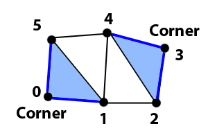
5.4. Identify all the triangles in the polygon

This step can be split in 2 stages: identifying the triangles of the polygon outline and identifying all the triangles enclosed by them. The input L for this step is the list of vertex indices of the outline we generated at the beginning of this section. Since we order the triangle vertices CCW, and we added the vertices of the new edges in the same order of the list, we can be sure that, for each edge E_P, the triangle that is inside the polygon is the one that has the 2 vertices in the order they are stored in the input list. This process will generate an output list of triangle indices.

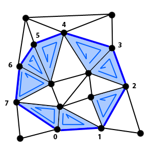
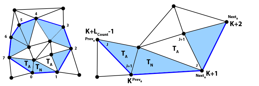
For each triangle T_N found in the mentioned way, we first check that it does not form a corner (2 consecutive edges in the outline) by comparing it to the last triangle added to the output list and also to the first one, since the polygon is closed (first edge and last edge are connected).

Then we get the 2 adjacent triangles T_A of T_N that do not share the current edge E_P and check whether such triangles have any of the edges in L that are contiguous to E_P. If K is the index of the first vertex in E_P, the vertices of such 2 contiguous edges are:

Prev_A = L[(K + L_COUNT – 1) % L_COUNT ]
Prev_B = L[K]
Next_A = L[(K + 1) % L_COUNT ]
Next_B = L[(K + 2) % L_COUNT ]

Remember that the polygon is closed so we need to wrap around L using the modulo operation. If J is the iterator (from 0 to 2) of the vertices of each triangle, then we check the following comparisons:

T_Av[J] == Prev_A AND T_Av[(J + 1) % 3] == Prev_B
OR
T_Av[J] == Prev_B AND T_Av[(J + 1) % 3] == Prev_A
OR
T_Av[J] == Next_A AND T_Av[(J + 1) % 3] == Next_B
OR
T_Av[J] == Next_B AND T_Av[(J + 1) % 3] == Next_A

Take into account that we are comparing the vertices of the edges of T_A in the opposite direction too, regarding the outline vertices. When 2 triangles are adjacent, the shared edge V₁ → V₂ in one triangle is V₂ → V₁ in the other. This occurs when the triangle is a corner and one of its adjacent triangles is outside of the polygon.

If T_A does not have an edge in the outline and it has not been added to the output list yet, then we add it to a stack of adjacent triangles that we can call S, to be processed later. Consider the previous comparisons as an optimization that avoids iterating through the output list always; instead, we only do it if T_A is not in the outline.

For the second stage, we propagate the quality of “being inside of the polygon” by adjacency until all the triangles that are not at the outline have been processed. While there are elements in S, we take a triangle out and check if it is already added to the output list. If that is the case, we ignore it and take the next one; otherwise, for each of its adjacent triangles we check whether it exists and whether it has not been added to the output list yet. If those conditions are met, we add it to S. Once the 3 adjacent triangles have been checked, we add the current triangle to the output list.

When this step finishes, we will have a list of indices of all the triangles that lay inside the polygon. We can use this list to remove or skip such triangles in a later step, leaving holes in our triangulation.

6. Supertriangle removal

The process ends when we remove the excess triangles that surround the main point cloud. Those triangles exist because we used a supertriangle as the first triangle of the set. It is easy to identify them, they all share at least one of the vertices of the supertriangle which, as you may deduce, are located at positions 0, 1 and 2 of the Points array. We just collect them by iterating through the triangle vertex array and store them in the list of triangles to remove.

7. Denormalization

If you normalized the input points, it is time to denormalize them. Use exactly the same bounding box calculated in the beginning for the main point cloud. For each point [X, Y] we get [X_D, Y_D]:

X_D = X * D_max + X_min
Y_D = Y * D_max + Y_min

8. Output filtering

We have the full triangulation, L, on one hand and the list of triangles to be removed, R, on the other. For each triangle in L, we check if it exists in R and, if it does, we remove it from R and check the next triangle; otherwise we add the triangle to the output list. Consider using a sorted list in previous steps, it may (or may not, measure it!) reduce the time spent in this process.

Known limitations

Although this algorithm works for the majority of the use cases, it has some limitations that are worth to mention:

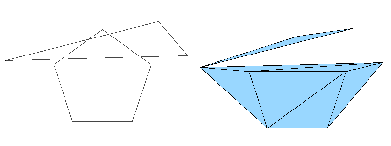
• The polygons that represent the holes cannot overlap each other. If you need some figures to intersect in order to form a figure, you should merge both polygons into one and use that “superpolygon” as a hole.

• If you use holes that are partially or totally out of the main point cloud, the part of the hole that lays outside may generate undesired new triangles that do not share any of the main points.

• If your points or holes are placed in such a way that very small triangles are formed, that may produce precision loss, which may lead to exceptions or freezing. You can mitigate this by not scaling the points by DMAX during normalization and denormalization steps.

• If points are added right on an existing edge, or if a constrained edge crosses exactly though an existing vertex, the process may fail. In order to avoid this, it is recommended to apply a tiny random offset to every point added to the triangulation, specially if constrained edges form figures with many orthogonal corners.

Code repository

https://github.com/QThund/ConstrainedDelaunayTriangulation

Final note: Thanks picolino0 for the bug fix.